
VLOOKUP in Google Sheets is a useful function for matching up data in different locations within a spreadsheet.
In this post, we’ll provide examples of how we used ChatGPT to simplify creating a VLOOKUP formula.
VLOOKUP: The Technical Explanation
The Google Sheets VLOOKUP function (as with Excel) is a vertical lookup function that searches for a value in a column or specified cell and returns a related value from another cell. The syntax for the VLOOKUP function is:
=VLOOKUP(search_key, range, index, [is_sorted])
- search_key is the value to search for in the first column of the range.
- range is the upper and lower values to consider for the search.
- index is the index of the column with the return value of the range. The index must be a positive integer.
- is_sorted is optional input. Options are:
- FALSE = Exact match. This is recommended by Google.
- TRUE = Approximate match. This is the default if is_sorted is unspecified.
A Less Technical Explanation
Here are the VLOOKUP parameters defined in narrative form.
The search key is the value you want to search for. For example, if you want to find the price for a particular product, the product name, number, or ID would be your search key.
The range is the array, a.k.a. table you want to search in. The table consists of at least two columns of data. The first column should contain the [possible] search key values. One of the columns should contain the values you want to return based on the search key.
The index is the column number (counting from the left of your defined array) of the value you want to return from the table. For example, if you want to return the price for a product from the third column of your range, your index value would be 3. This is the column in which the vertical lookup is performed.
Sorted is an optional input that specifies whether you want an exact match or an approximate match for your search_key value. If you enter “FALSE”, the function will look for an exact match. If you enter “TRUE,” the function will look for the closest match to your search key value.
Example Business Uses of VLOOKUP
Rather than creating our formula manually, we prompted ChatGPT for a VLOOKUP formula. Here are the results.
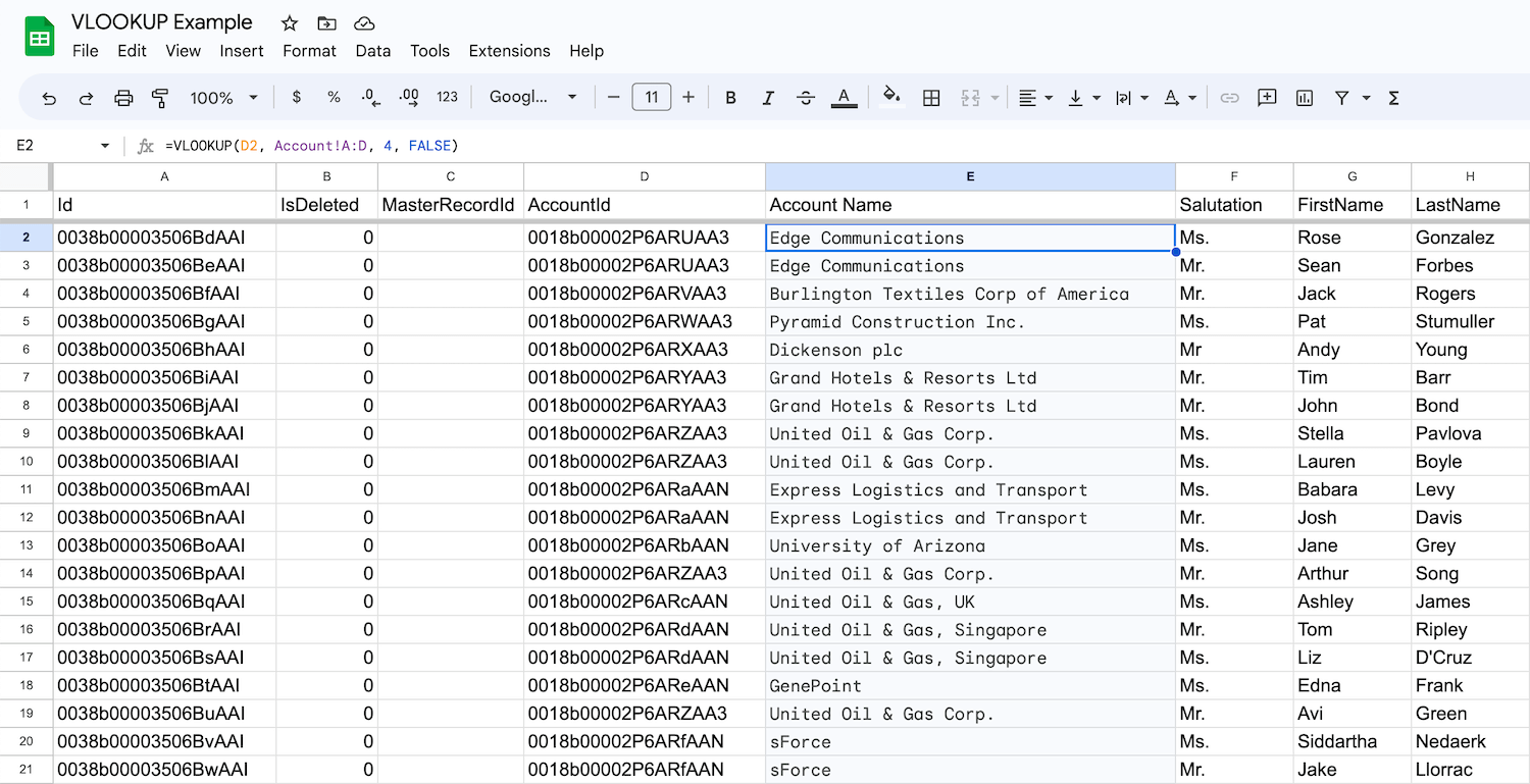
Salesforce Contact Export Example
If you do a raw export of Salesforce Contact information, the export file contains the parent Account ID, but not the contact’s Account Name.
So, we exported the Salesforce Contact and Account information and imported the resulting CSVs into separate sheets in the same Google Sheets file.
Here is the prompt we fed ChatGPT.
I have a Google Sheet with two sheets – Contact and Account. In the Contact sheet, the Account IDs are in Column D. I want to use a VLOOKUP formula to find the Account Name for each contact in the Account sheet. In the Account sheet, the Account IDs are in Column A. The Account Names are in Column D. Please create a VLOOKUP formula.
ChatGPT returned the formula =VLOOKUP(D2, Account!A:D, 4, FALSE)
Based on the ChatGPT’s response we added a new column E to the Contact sheet and pasted its suggested formula in cell E2. Google Sheets auto-suggested a fill-down of column E, which we accepted.
Here is ChatGPT’s explanation of its formula (=VLOOKUP(D2, Account!A:D, 4, FALSE)).
In this formula:
D2 is the cell containing the Account ID in the Contact sheet.
- Account!A:D is the range of cells in the Account sheet where the lookup will be performed. The first column of this range (Column A) contains the Account IDs, and the fourth column (Column D) contains the Account Names.
- 4 is the index of the column (in the range Account!A:D) that contains the Account Name. Since the Account Names are in Column D, which is the fourth column in the range, we use the number 4 here.
- FALSE specifies that we want an exact match for the Account ID. If there is no exact match, VLOOKUP will return an error.
Copy this formula down for all the rows in the Contact sheet where you want to retrieve the Account Name, and it will automatically look up the corresponding Account Name for each Contact based on their Account ID.
Tip: if you want to replace the formula references in Column E with values, select and copy the entire column. Then, paste over it by selecting ‘Paste special > Values only.’
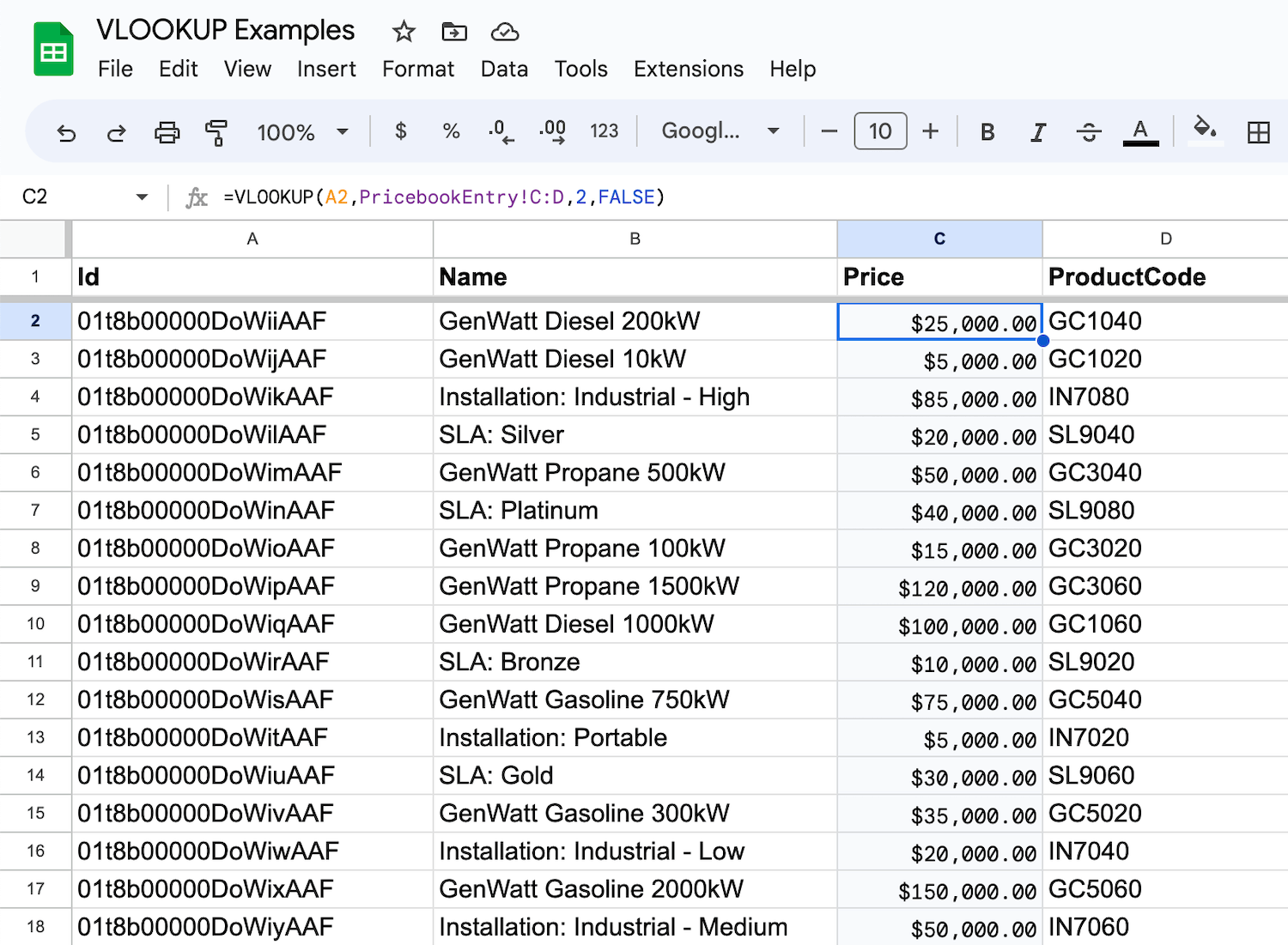
Salesforce Product & Pricebook Export
A raw export of the Salesforce Product object data does not show a price — only a Pricebook ID. Prices are in the PricebookEntry object export.
So, our ChatGPT prompt was:
I have a spreadsheet with two sheets – Product2 and PricebookEntry. In Product2, the product IDs are in Column A. I want to use a VLOOKUP formula to find the price for each product in the PricebookEntry sheet. In the PricebookEntry sheet, the Product2 IDs are in Column C. The prices are in Column D. Please create a VLOOKUP formula.
ChatGPT returned the formula =VLOOKUP(A2,PricebookEntry!C:D,2,FALSE)
We added a new column C to the Product export and pasted the VLOOKUP formula into cell C2 and then dragged the values down for all products.
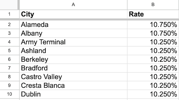
Sales tax by California ZIP Code
This is an example of how to create a list of sales tax rates by ZIP Code for billing purposes.
We first downloaded a list of California sales tax rates by city and uploaded it to the first sheet of a Google Sheets file.
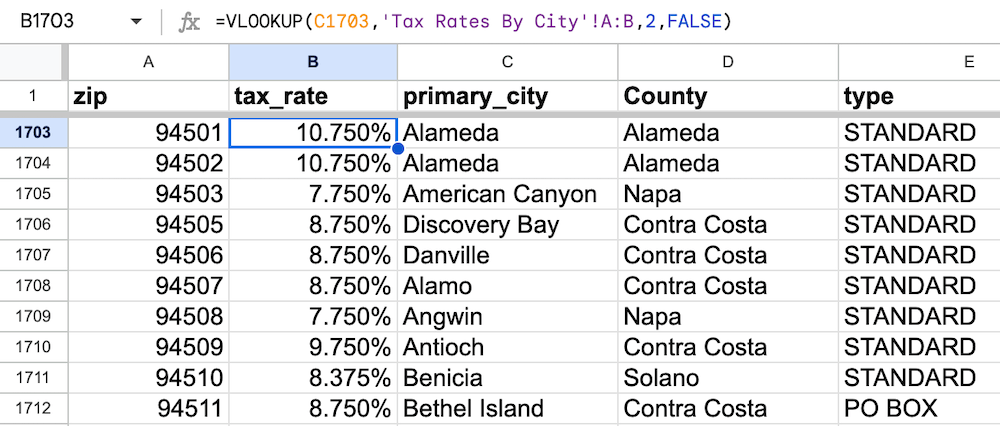
We then downloaded a list of all U.S. ZIP Codes and uploaded it to the second sheet of the same Google Sheets file.
We used the VLOOKUP formula =VLOOKUP(C2,’Tax Rates By City’!A:B,2,FALSE) to get a column of tax rates by ZIP Code.
We hope you find these business examples useful, including how to prompt ChatGPT for a VLOOKUP formula.