Update: on December 8, 2022, Google introduced drop-down chips in Google Sheets, which vastly simplifies the process described below.
One aspect of spreadsheets that makes them different from database applications is that it’s more difficult to enforce data entry standards in spreadsheets.
By default, entries into unlocked cells in Google Sheets care freeform. You and any editors you share a Sheet with can type or paste any numbers, letters, symbols, or image into an unlocked cell.
But it is possible to enforce user entry of specific values in certain Google Sheets cells by adding in-cell dropdown lists.
Steps for creating and using dropdown lists
Our recommended approach is to first create a new sheet within an existing Google Sheets file. Name the sheet “Dropdown Values.”
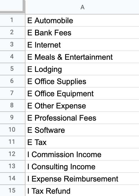
We’ll use business income and expense accounts as an example.
Add income and expense values to Column A. We have entered values in the A1 to A15 range.
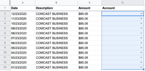
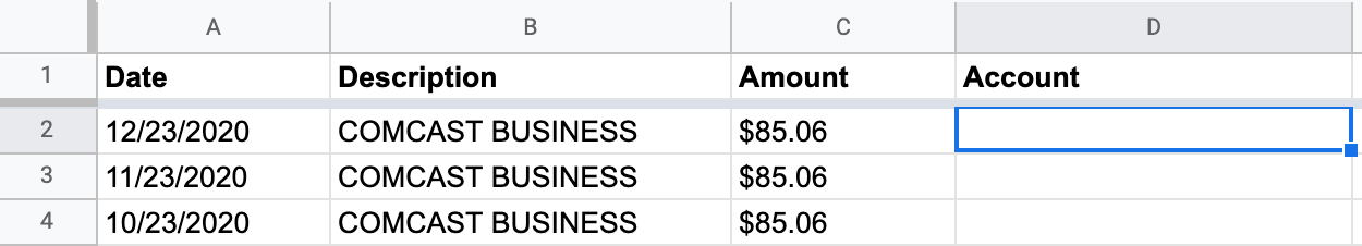
In a separate sheet within the same file used to track income and expense line items, add a column with a header name of “Account.”
Select the cell under the column header.
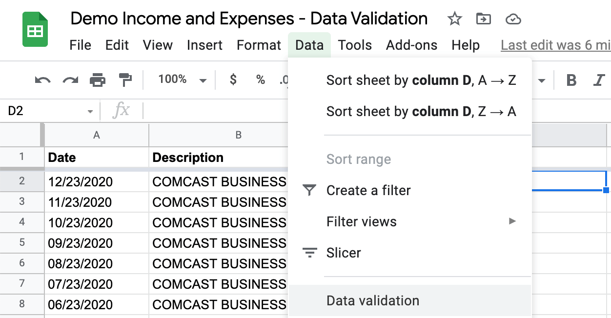
Add data validation to this cell by selecting Data > Data validation from the menus.
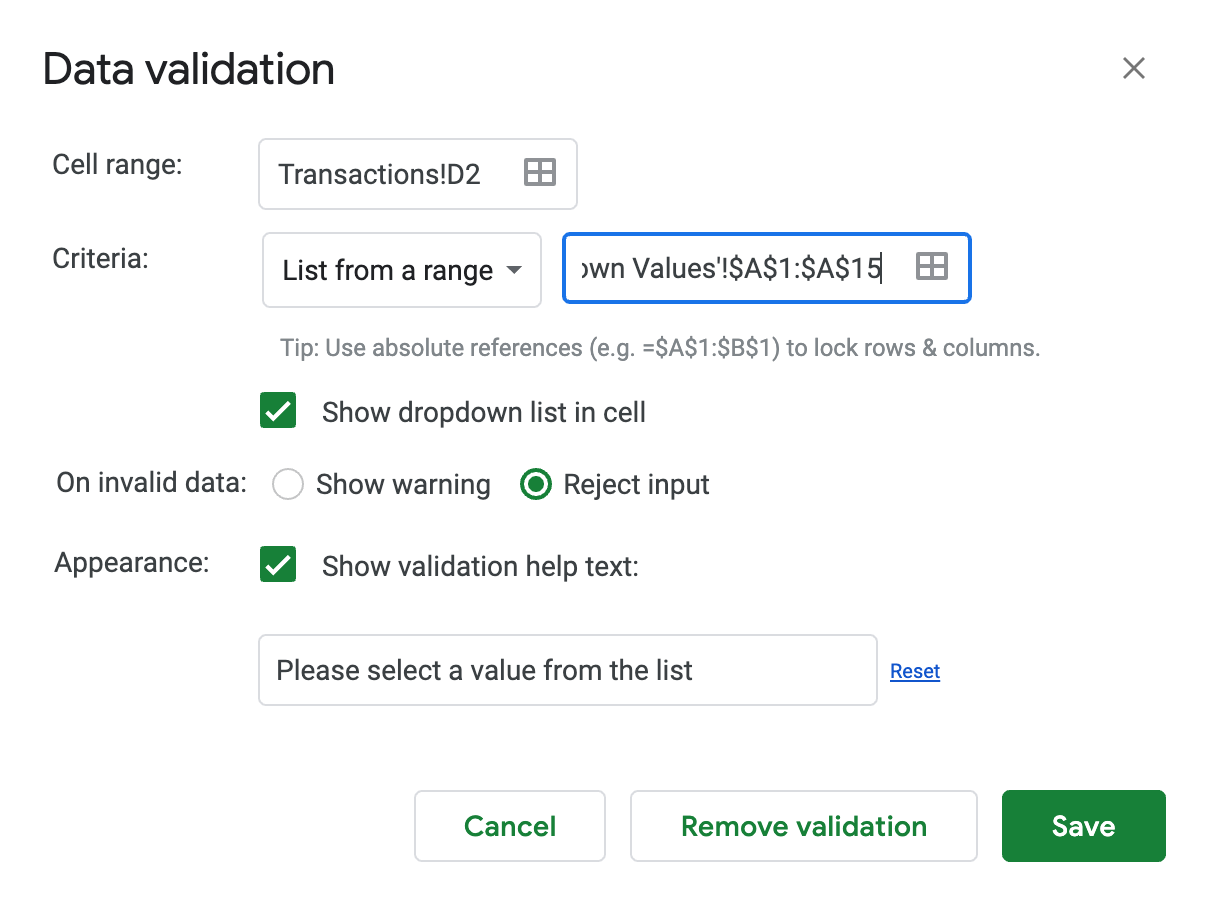
In the Data validation dialog:
- Select the “List from a range” criteria
- Enter the range using =’Dropdown Values’!$A$1:$A$15
- Click the “Show dropdown list in a cell” checkbox option
- Select the “Reject input” radio button (the “Show warning” selection will allow users to enter a value that is not in the list)
- Click the “Show validation help text:” checkbox
- Add help text such as “Please select a value from the list”
- Click the Save button
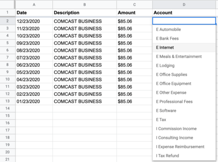
When you click into the cell, you will see the dropdown list. Make a selection from the list of options.
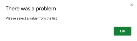
If a Sheet editor types something into the cell rather than selecting a value from the list, they will see the following dialog.
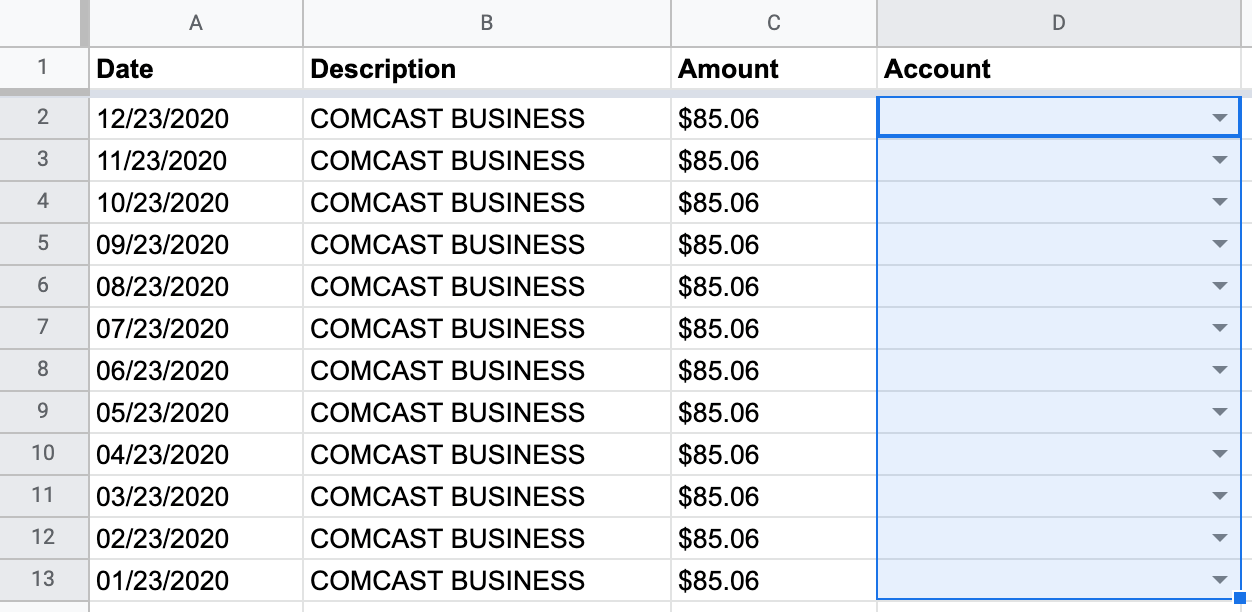
The last step is to copy down cell D2 through to as many cells as needed. You can also copy down a cell after making a selection, which is convenient when you have sorted the sheet by Column B, as we have in this example.
You are now ready to use the dropdown list for yourself and other editors of the Google Sheet.
Keep in mind that you can create more than one drop-down list in a single spreadsheet.